Interpreting Skew-Ts (Part One)

Now that the basics of a Skew-T are understood, we can now talk about how to put all of it together, and learn how to interpret a Skew-T.  It’s important to have a firm grasp on what the parts of a Skew-T mean before continuing into this section.

One of the most frequently asked questions when reading a Skew-T and interpreting the information is, how do you know if air will rise or not, thus be unstable or stable?  The answer to this question is very simple – there’s one more line that is drawn on a Skew-T that was not described (although mentioned) before.  That is the Theoretical Air Parcel Plot line (TAPP).  This is the grey line that can be seen on the Skew-T.  This indicates how a parcel of air will move, however it is imperative that the word theoretical is taken into account.  As with many applications of meteorology, what works in theory does not always work in a practical situation.  This will be explored in the next section further.

If the TAPP lies to the right of the temperature line (environmental lapse rate, or the ELR), then that section of the atmosphere is unstable... 

If the TAPP lies to the left of the temperature line, then that section of the atmosphere is stable...

Remembering that the Theoretical Air Parcel Plot line informs you how a parcel of air will rise in the atmosphere.  Basically, it tells you the temperature at which it’ll proceed if it’s allowed to rise in the atmosphere.  So if the temperature if the TAPP is warmer than the ELR, then it’ll become positively buoyant and rise past that point (if allowed to reach that point).  It’s warmer, because if you read the temperature along the horizontal axis, you’ll see that the TAPP will achieve a higher temperature then the ELR. 

If the temperature at the TAPP is cooler than the ELR, then it’ll become negatively buoyant.  This does not necassarily mean it will not rise past this point though, and this will be explained in the next section.  It will either slow down, or not be allowed past this point. 

However – it is not quite as easy as this all the time.  Quite often, we have times when the atmosphere has inversions, caps or sometimes the atmosphere is conditionally unstable, or completely unstable.  Below, is an example of different Skew-T’s and an explanation on “deciphering” them for the relevant information to “read” what the atmosphere is doing.

There is one small section where the air parcel is slightly warmer then the ELR however, up until around the 850mb, so we might expect some very small Cu (probably stratocumulus!)  But then no other convective clouds above that level as the atmosphere goes from marginally unstable, to strongly stable, and this layer will prevent any air from rising.

A few other comments that can be made, is the dryness of the overall atmosphere.  Notice how far the DP and the temperature lines are apart?  This is a sign of a dry atmosphere.  The further the DP and the temperature lines are apart, the drier the atmosphere.  Sometimes you can have differing moist and dry layers throughout the atmosphere, during that case you’ll see the DP line ‘jump’ around a fair bit, but you’ll distinctly see moist and dry layers.

Another feature on this is the presence of a large inversion in the upper levels (between the 250mb and the 200mb levels).  An inversion is vertical section of the atmosphere where the temperature increases with height.  You can see the that the 250mb temperature is approximately –59C.  But the 200mb temperature, is –54C.  So the temperature has increased with height, and this is therefore an inversion.  The size and strength of the inversion depends on how sharply the temperature line veers to the right (temperature gradient increase), and for how long it does so (the size of the inversion).  Another inversion is present between 850mb and 800mb which actually commences the start of our stable layer!

Lets look at another example, only this is a different Skew-T.  Well, not really different - just different colours and format, it still tells you the same.  It's just that this particular situation I want to illustrate is quite rare, and I saved this image back in 1998 when the BoM soundings weren't available.  If you really have trouble understanding, I've written a quick page introducing the colour scheme of this particular Skew-T here.

A cap is considered as a ‘lid’ on convection.  A cap is an area where the TAPP crosses to the left of the ELR, and then eventually crosses back to the right of the ELR.  So in between, you’ll have an area of stability that suppresses convection.  A cap is not to be confused with an inversion, which is simply a descriptive term on what the ELR does, it has nothing to do with the TAPP.  However, because of an inversion’s properties, a cap often occurs near, or on an inversion.  This is a reason why these two terms are often confused to have analogous meanings.

This may now become a little confusing, as if the cap is a stable layer, and the particular sounding used in this example is a representation of a completely unstable atmosphere, how is the atmosphere completely unstable?  There’s are few other things that must be noted when looking at instability.  The larger the difference between the TAPP and the ELR, then the stronger the stability, or instability is in that area.  For example, if a parcel of air is 5C warmer than its surroundings, it’ll ascend faster than air that is 2C warmer than its surroundings.  Here's what I mean:

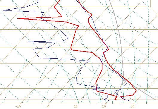
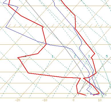
Both of these parts of the atmosphere are unstable, but the one on the right is more unstable than the left.  That can be seen even just looking at the LIs.  -4 LIs on the first sounding vs -9 LIs on the second sounding.

Similarly, if air is 5C colder than its surroundings, it’ll descend OR reduce speed faster than a parcel of air 2C colder.  As air rises, it gains momentum, updrafts can often gain speed very quickly, reaching 40-60km/h and sometimes as high as 150km/h.  When an updraft, or a parcel of air that is ascending reaches a stable layer (eg, a cap), it begins to slow down, but it doesn’t stop immediately.  A useful analogy that can be used, is the example of a ball rolling down a hill.  The steep the decline (the warmer the parcel of air is to its surroundings), the faster the ball will roll down the hill (the faster the parcel of air will ascend).  The opposite can occur when a ball rolling down a slope, reaches an incline.  What happens when a ball rolling down a slope suddenly reaches an incline?  Will it stop immediately?  It certainly will not!  It’ll roll up the incline and slow down.  The steeper the incline, the faster the ball will slow down (the faster a parcel of air will reduce its speed), and if a ball is placed at the bottom of an incline, it simply won’t move at all (a parcel of air will not ascend, therefore is stable).

The small cap that can be seen on the sounding will easily be ‘broken’ from the momentum of air gained from below it, where it’s slightly unstable.  Basically, this stable layer is so negligible, that in our rolling ball example, this will be seen as a very small incline on a declining slope.  The ball would have been given an opportunity to already gain speed, and will slow down at the incline, but still proceed over the incline, and will travel down the rest of the slope without hinderence.  Similarly, our parcel of air that is rising in the atmosphere that this skew-T represents will see this cap as a small hindrance, and will slow down at this point, and continue rising. For this reason, small caps in the lower atmosphere are easily broken – often without any other assistance.  Now you can understand why before, the cap mentioned in the Skew-T could easily be broken, as the air gathered momentum, it was able to break such a small cap.  Anything under 0.5C can easily be broken by this method. 

Here is a good place to introduce CAPE, (Convective Available Potential Energy).  CAPE is, as the name suggests, the amount of available convective potential energy in the atmosphere.  Crudely, but simply – it is the measure of the area between the air parcel line and the ELR where the air parcel is to the right of the ELR.  The larger the CAPE, the more unstable the atmosphere is.  Air will rise faster if it is significantly warmer then its surroundings, this results in stronger, and more sustained updrafts.  With CAPE being a measure of this instability, it is fairly explanatory why large CAPE’s often correspond with severe thunderstorm development. 

Think of CAPE this way in regards to the atmosphere.  If CAPE is simply a measure of the amount of area that the air parcel line lies to the right of the ELR, then the larger the CAPE the larger the temperature differences between these two lines.  Time for some more examples, lets look at two soundings - both having large areas of instability, but one being more unstable than the other.

Anyway, back to CAPE - I said the second sounding had more CAPE than the first...I better give some proof of that, here are the figures:

As you can see, there's much more CAPE in the second sounding compared to the first!  Hopefully that helps give you an idea and a concept about what CAPE is!  I'll give a set of "magic numbers" for CAPE too.  Keep in mind that, you can get tornadic supercells in CAPE of just 100-200 in the right conditions!  If you continue to read on in this guide, you'll discover why.  I've also included some typical LI values you might see with these CAPEs.  Keep in mind that while there is a correlation with CAPE and LI values, there can be significant differences!  Hence there is some overlap in the figures.  These magic numbers are assuming the cap breaks:
 
 

We have now seen two examples of skew-T’s representing completely stable, and completely unstable atmospheres.  However, more often the not, we’ll see that the atmosphere is neither.  Sometimes the atmosphere is unstable in the lower levels, but stable in the upper levels (eg, low-mid topped showers).  Unstable in the mid-upper levels, but very stable in the low levels (generally sunny, occasionally some Altocumulus Castellatus).  Or sometimes it’s generally unstable, but stable in other areas – all of these give differing results.  But importantly, we have to remember that a skew-T is a vertical slice of the atmosphere at the time the sounding was taken.  During that time, a myriad of factors can change, cold air can come through in the upper levels, or an upper level ridge may move through.  Alternatively, moisture in the upper levels may suddenly increase or decrease.  But the most common change that occurs is the change at the surface.  The change that results in the surface conditions is often so great that it frequently alters what a seemingly stable, or unstable atmosphere will actually produce.  So how can the skew-T be adjusted to represent the change in at the surface?  It’s quite simple, but rather long-winded and is explained in the next section.